


MAT 275 CHAPTER 6, 7 PRACTICE PROBLEMS
(Material from earlier sections are on previous reviews)
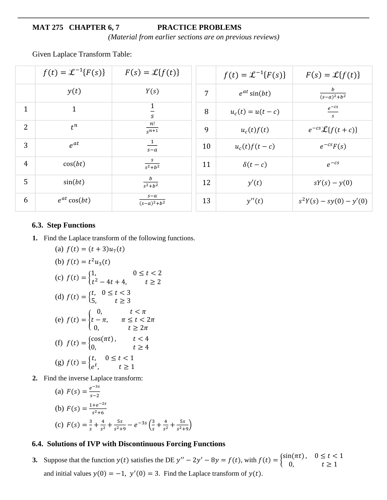
Given Laplace Transform Table:
6.3. Step Functions
1. Find the Laplace transform of the following functions.
(a) 𝑓(𝑡)=(𝑡+3)𝑢7(𝑡)
(b) 𝑓(𝑡)=𝑡2𝑢3(𝑡)
(c) 𝑓(𝑡)={1, 0≤𝑡<2
𝑡2− 4𝑡 + 4, 𝑡≥2
(d) 𝑓(𝑡)={𝑡, 0≤𝑡<3
5, 𝑡≥3
(e) 𝑓(𝑡)={0,
𝑡−𝜋,
0, 𝑡<𝜋
𝜋≤𝑡<2𝜋
𝑡≥2𝜋
(f) 𝑓(𝑡)={cos(𝜋𝑡), 𝑡<4
0, 𝑡≥4
(g) 𝑓(𝑡)={𝑡, 0≤𝑡<1
𝑒𝑡, 𝑡≥1
2. Find the inverse Laplace transform:
(a) 𝐹(𝑠)=𝑒−3𝑠
𝑠−2
(b) 𝐹(𝑠)=1+𝑒−2𝑠
𝑠2+6
(c) 𝐹(𝑠)=3
𝑠+4
𝑠2+5𝑠
𝑠2+9−𝑒−3𝑠(3
𝑠+4
𝑠2+5𝑠
𝑠2+9)
6.4. Solutions of IVP with Discontinuous Forcing Functions
3. Suppose that the function 𝑦(𝑡) satisfies the DE 𝑦′′−2𝑦′−8𝑦=𝑓(𝑡), with 𝑓(𝑡)={sin(𝜋𝑡), 0≤𝑡<1
0, 𝑡≥1
and initial values 𝑦(0)=−1, 𝑦′(0)=3. Find the Laplace transform of 𝑦(𝑡).
𝑓(𝑡)= ℒ{𝐹(𝑠)}
−1
𝐹(𝑠)= ℒ{𝑓(𝑡)}
𝑦(𝑡)
𝑌(𝑠)
1
1
1
𝑠
2
𝑡𝑛
𝑛!
𝑠𝑛+1
3
𝑒𝑎𝑡
1
𝑠−𝑎
4
cos(𝑏𝑡)
𝑠
𝑠2+𝑏2
5
sin(𝑏𝑡)
𝑏
𝑠2+𝑏2
6
𝑒𝑎𝑡cos(𝑏𝑡)
𝑠−𝑎
(𝑠−𝑎)2+𝑏2
𝑓(𝑡)= ℒ{𝐹(𝑠)}
−1
𝐹(𝑠)= ℒ{𝑓(𝑡)}
7
𝑒𝑎𝑡sin(𝑏𝑡)
𝑏
(𝑠−𝑎)2+𝑏2
8
𝑢𝑐(𝑡)=𝑢(𝑡−𝑐)
𝑒−𝑐𝑠
𝑠
9
𝑢𝑐(𝑡)𝑓(𝑡)
𝑒−𝑐𝑠ℒ{𝑓(𝑡+𝑐)}
10
𝑢𝑐(𝑡)𝑓(𝑡−𝑐)
𝑒−𝑐𝑠𝐹(𝑠)
11
𝛿(𝑡−𝑐)
𝑒−𝑐𝑠
12
𝑦′(𝑡)
𝑠𝑌(𝑠)−𝑦(0)
13
𝑦′′(𝑡)
𝑠2𝑌(𝑠)−𝑠𝑦(0)−𝑦′(0)
4. Consider the following IVP: 𝑦′′+16𝑦=2−2𝑢3(𝑡), 𝑦(0)=0, 𝑦′(0)=0.
(a) Find the Laplace transform of the solution 𝑦(𝑡).
(b) Find the solution 𝑦(𝑡) by inverting the transform.
6.5. Impulse Functions
5. A mass 𝑚 =1 is attached to a spring with constant 𝑘 =5 and damping constant 𝑐 = 2. At the instant
𝑡=𝜋, the mass is struck with a hammer, providing an impulse 𝑝 = 10. Also, 𝑥(0)=0 and 𝑥′(0)=0.
a) Write the differential equation governing the motion of the mass.
b) Find the Laplace transform of the solution x(t).
c) Apply the inverse Laplace transform to find the solution.
6. Consider the following IVP: 𝑦′′+ 4𝑦=5𝛿(𝑡− 3), 𝑦(0)=1, 𝑦′(0)=2.
(a) Find the Laplace transform of the solution 𝑦(𝑡).
(b) Find the solution 𝑦(𝑡) by inverting the transform.
7.1. Introduction to Systems
7. Transform the given IVP into an initial value problem for two first order equations.
(a) 𝑦′′−6𝑦′+8𝑦=0
(b) 𝑢′′+4𝑢′+5𝑡𝑢=7−sin(2𝑡)
8. Write the following IVP for a system of two linear ODEs as an IVP for a single second-order ODE.
(a) 𝑥′=−𝑦 𝑥(0)=1
𝑦′=10𝑥 − 7𝑦 𝑦(0)=−7
(b) Solve the above IVP
9. Match the description of the phase portrait with the corresponding system (one description will not match).
I 𝑥′=𝑦, 𝑦′=−𝑥 II 𝑥′=𝑦,𝑦′=𝑥 III 𝑥′=−2𝑦, 𝑦′=𝑥
A. circles B. ellipses C. hyperbolas D. parallel lines
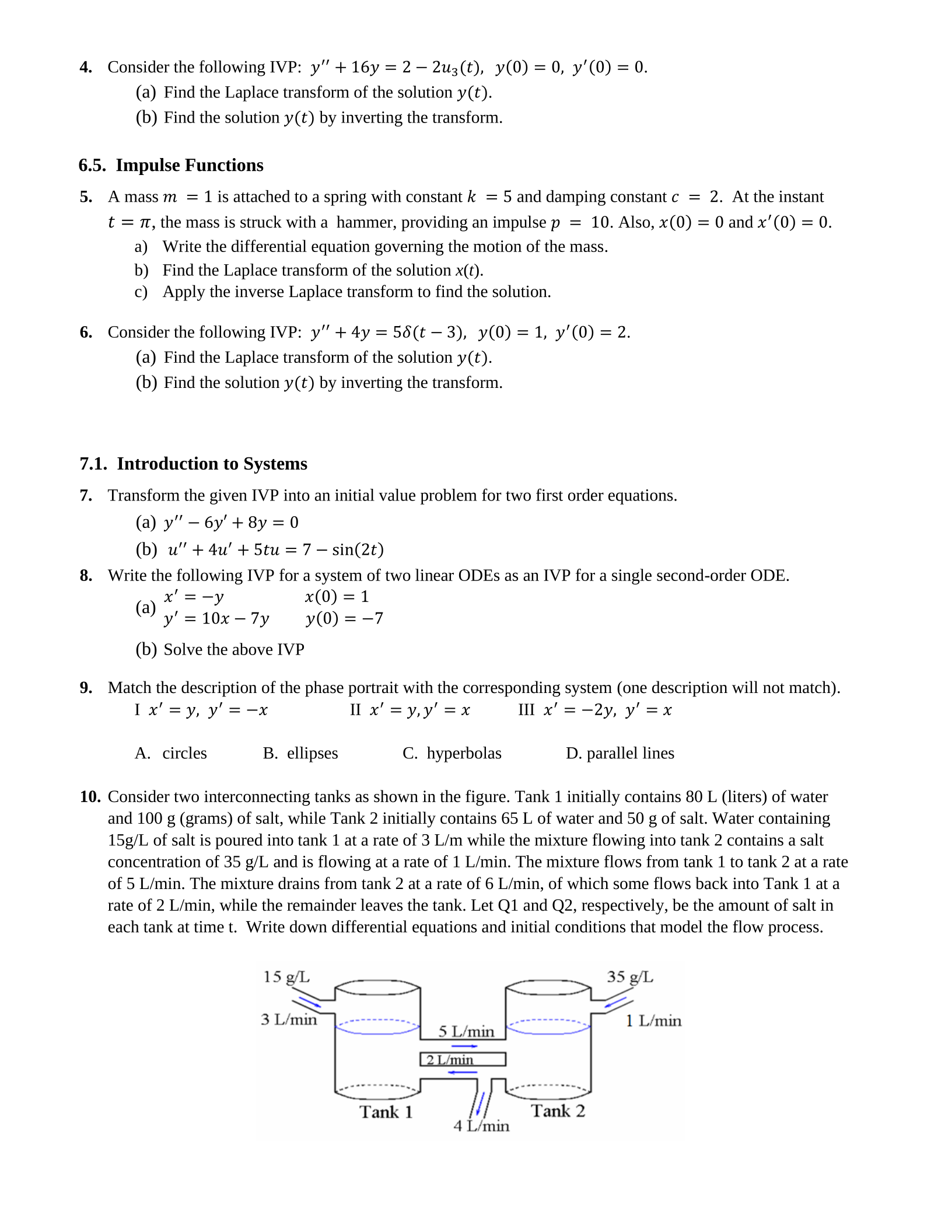
10. Consider two interconnecting tanks as shown in the figure. Tank 1 initially contains 80 L (liters) of water
and 100 g (grams) of salt, while Tank 2 initially contains 65 L of water and 50 g of salt. Water containing
15g/L of salt is poured into tank 1 at a rate of 3 L/m while the mixture flowing into tank 2 contains a salt
concentration of 35 g/L and is flowing at a rate of 1 L/min. The mixture flows from tank 1 to tank 2 at a rate
of 5 L/min. The mixture drains from tank 2 at a rate of 6 L/min, of which some flows back into Tank 1 at a
rate of 2 L/min, while the remainder leaves the tank. Let Q1 and Q2, respectively, be the amount of salt in
each tank at time t. Write down differential equations and initial conditions that model the flow process.
7.2-7.4. Matrices, Basic Theory of Systems
11. Verify that 𝐱=[1
0]𝑒𝑡+[2
2]𝑡𝑒𝑡 is a solution of the system 𝐱′=[2 −1
3 −2]𝐱+[1
−1]𝑒𝑡.
12. Given the system 𝑥′=𝑡𝑥−𝑦+𝑒𝑡𝑧, 𝑦′=2𝑥+𝑡2𝑦−𝑧, 𝑧′=𝑒−𝑡+3𝑡𝑦+𝑡3𝑧, define 𝐱, 𝑃(𝑡) and 𝐟(𝑡)
such that the system is represented as 𝐱′=𝑃(𝑡)𝐱+𝐟(𝑡).
13. Consider the second order initial value problem 𝑢′′+2𝑢′+2𝑢=3sin(𝑡), 𝑢(0)=2,𝑢′(0)=−1. Change
the IVP into a first order initial value system and write the resulting system in matrix form.
14. Are the vectors 𝐱𝟏=[1
−1
1], 𝐱𝟐=[0
1
1] , 𝐱𝟑=[1
1
1] linearly independent?
15. Consider the system 𝐱′=[−2 −6
0 1]𝐱. Two solutions are 𝐱𝟏=[−2
1]𝑒𝑡 and 𝐱𝟐=([1
0])𝑒−2𝑡.
(a) Use the Wronskian to verify that the two solutions are linearly independent.
(b) Write the general solution of the system.
16. Suppose the system 𝐱′=𝐴𝐱 has general solution 𝐱(𝑡)=𝑐1[−2
1
0]𝑒𝑡+𝑐2 [1
0
1]𝑒−2𝑡+𝑐3[0
1
1]𝑒−𝑡, where
𝐱(𝑡)=[𝑥1(𝑡)
𝑥2(𝑡)
𝑥3(𝑡)]. Given the initial condition 𝐱(𝑡)=[1
1
−1], find 𝑥1(𝑡), 𝑥2(𝑡), and 𝑥3(𝑡).
7.5. Homogeneous Linear Systems with Constant Coefficients; Real, Distinct Eigenvalues
17. Solve the IVP 𝐱′=𝐴𝐱 with 𝐴=[1 −3
0 −2] and 𝒙(0)=[1
3].
18. Solve the IVP 𝑥′=𝑥+2𝑦
𝑦′=4𝑥+3𝑦 with 𝑥(0)=3, 𝑦(0)=0.
7.6. Homogeneous Linear Systems with Constant Coefficients; Complex Eigenvalues
19. Find the general solution to 𝐱′=𝐴𝐱 with 𝐴=[1 −2
4 −3].
20. Solve the IVP 𝑥′=𝑥+2𝑦
𝑦′=−5𝑥−𝑦 with 𝑥(0)=4, 𝑦(0)=1.
21. Suppose 𝐴 is real 3×3 matrix that has the following eigenvalues and eigenvectors:
−2,[1
1
1], 1+𝑖,[1−𝑖
2
1], 1−𝑖,[1+𝑖
2
1]. Find a fundamental set of real valued solutions to 𝐱′=𝐴𝐱.
7.8. Homogeneous Linear Systems with Constant Coefficients; Repeated Eigenvalues
22. Find the general solution to 𝐱′=𝐴𝐱 with 𝐴=[−5 9
−1 1].
23. Solve the IVP 𝑥′=4𝑥+ 3𝑦
𝑦′=−3𝑥−2𝑦 with 𝑥(0)=1, 𝑦(0)=−2.
ANSWERS TO CHAPTER 6-7 PRACTICE PROBLEMS
6.3. Step Functions
1. (a) L{𝑓(𝑡)}=𝑒−7𝑠 L{𝑡+10}=𝑒−7𝑠(1
𝑠2+10
𝑠)
(b) L{𝑓(𝑡)}=𝑒−3𝑠L{(𝑡+3)2}=𝑒−3𝑠L{𝑡2+6𝑡+9}=𝑒−3𝑠(2
𝑠3+6
𝑠2+9
𝑠)
(c) 𝑓(𝑡)=1+𝑢2(𝑡)(𝑡2−4𝑡+3) so L{𝑓(𝑡)}=1
𝑠+𝑒−2𝑠L{(𝑡+2)2−4(𝑡+2)+3}
=1
𝑠+𝑒−2𝑠L{𝑡2−1}=1
𝑠+𝑒−2𝑠(2
𝑠3−1
𝑠)
(d) 𝑓(𝑡)=𝑡−𝑢3(𝑡)(𝑡−5) so L{𝑓(𝑡)}=1
𝑠2−𝑒−3𝑠L{𝑡+3−5} =1
𝑠2−𝑒−3𝑠(1
𝑠2−2
𝑠)
(e) 𝑓(𝑡)=𝑢𝜋(𝑡)(𝑡−𝜋)−𝑢2𝜋(𝑡)(𝑡−𝜋) so L{𝑓(𝑡)}= 𝑒−𝜋𝑠L{(𝑡+𝜋)−𝜋}
−𝑒−2𝜋L{(𝑡+2𝜋)−𝜋} =𝑒−𝜋𝑠L{𝑡}−𝑒−2𝜋L{𝑡+𝜋} =𝑒−𝜋𝑠
𝑠2−𝑒−2𝜋𝑠(1
𝑠2+𝜋
𝑠)
(f) 𝑓(𝑡)=cos(𝜋𝑡)−𝑢4(𝑡)cos(𝜋𝑡) so L{𝑓(𝑡)}=𝑠
𝑠2+𝜋2−𝑒−4𝑠L{cos(𝜋(𝑡+4))}
=𝑠
𝑠2+𝜋2− 𝑒−4𝑠L{cos(𝜋𝑡)cos(4𝜋)−sin(𝜋𝑡)sin(4𝜋)}
=𝑠
𝑠2+𝜋2−𝑒−4𝑠L{cos(𝜋𝑡)}=𝑠
𝑠2+𝜋2− 𝑠𝑒−4𝑠
𝑠2+𝜋2
(g) 𝑓(𝑡)=𝑡+𝑢1(𝑡)(𝑒𝑡−𝑡) so L{𝑓(𝑡)}= 1
𝑠2+𝑒−𝑠L{𝑒𝑡+1−(𝑡+1)}
=1
𝑠2+𝑒−𝑠(𝑒
𝑠−1−1
𝑠2−1
𝑠)
2. (a) The inverse Laplace transform is 𝑢3(𝑡)𝑓(𝑡−3) where 𝑓(𝑡)= L{1
𝑠−2}
−1 =𝑒2𝑡
Thus L{𝑒−3𝑠
𝑠−2}
−1 =𝑢3(𝑡)𝑒2(𝑡−3).
(b) 𝐹(𝑠)=1
√6√6
𝑠2+6+𝑒−2𝑠
√6√6
𝑠2+6, thus L{𝐹(𝑠)}
−1 =1
√6sin(√6 𝑡)+1
√6𝑢2(𝑡)sin(√6(𝑡−2))
(c) L{𝐹(𝑠)}
−1 =3+4𝑡+5cos(3𝑡)−𝑢3(𝑡)(3+4(𝑡−3)+5cos(3(𝑡−3)))
6.4. Solutions of IVP with Discontinuous Forcing Functions
3. 𝑌(𝑠)=−𝑠+5
𝑠2−2𝑠−8+𝜋
(𝑠2−2𝑠−8)(𝑠2+𝜋2)+𝑒−𝑠 𝜋
(𝑠2−2𝑠−8)(𝑠2+𝜋2)
4. (a) 𝑌(𝑠)=2
𝑠(𝑠2+16)−𝑒−3𝑠 2
𝑠(𝑠2+16)=1
8(1
𝑠)−1
8(𝑠
𝑠2+16)−𝑒−3𝑠(1
8(1
𝑠)−1
8(𝑠
𝑠2+16))
(b) 𝑦(𝑡)=1
8−1
8cos(4𝑡)−𝑢3(𝑡)(1
8−1
8cos(4(𝑡−3)))
6.5. Impulse Functions
5. (a) 𝑥′′+2𝑥′+5𝑥=10𝛿(𝑡−𝜋) (b) 𝑋(𝑠)=10𝑒−𝜋𝑠
(𝑠+1)2+4
(c) 𝑥(𝑡)=5𝑢𝜋(𝑡)𝑒−(𝑡−𝜋)sin(2(𝑡−𝜋))=5𝑢𝜋(𝑡)𝑒−(𝑡−𝜋)sin(2𝑡)
6. (a) 𝑌(𝑠)=𝑠+2
𝑠2+4+5𝑒−3𝑠 1
𝑠2+4 (b) 𝑦(𝑡)=cos(2𝑡)+sin(2𝑡)+5
2𝑢3(𝑡)sin(2(𝑡−3))
7.1. Introduction to Systems
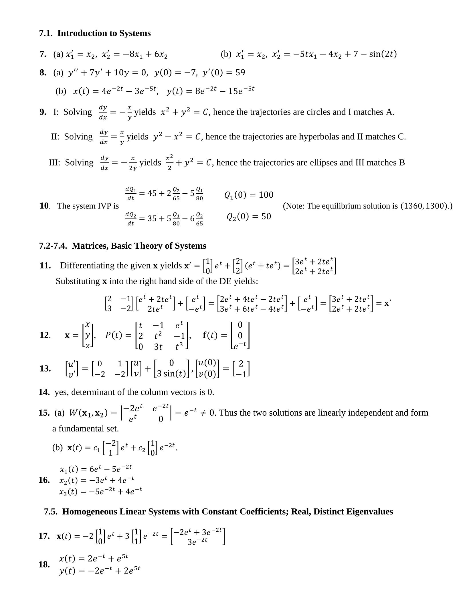
7. (a) 𝑥1
′=𝑥2, 𝑥2
′=−8𝑥1+6𝑥2(b) 𝑥1
′=𝑥2, 𝑥2
′=−5𝑡𝑥1−4𝑥2+7−sin(2𝑡)
8. (a) 𝑦′′+7𝑦′+10𝑦=0, 𝑦(0)=−7, 𝑦′(0)=59
(b) 𝑥(𝑡)=4𝑒−2𝑡−3𝑒−5𝑡, 𝑦(𝑡)=8𝑒−2𝑡−15𝑒−5𝑡
9. I: Solving 𝑑𝑦
𝑑𝑥=−𝑥
𝑦yields 𝑥2+𝑦2=𝐶, hence the trajectories are circles and I matches A.
II: Solving 𝑑𝑦
𝑑𝑥=𝑥
𝑦yields 𝑦2−𝑥2=𝐶, hence the trajectories are hyperbolas and II matches C.
III: Solving 𝑑𝑦
𝑑𝑥=−𝑥
2𝑦 yields 𝑥2
2+𝑦2=𝐶, hence the trajectories are ellipses and III matches B
10. The system IVP is 𝑑𝑄1
𝑑𝑡 =45+2𝑄2
65−5𝑄1
80
𝑑𝑄2
𝑑𝑡 =35+5𝑄1
80−6𝑄2
65
𝑄1(0)=100
𝑄2(0)=50 (Note: The equilibrium solution is (1360,1300).)
7.2-7.4. Matrices, Basic Theory of Systems
11. Differentiating the given 𝐱 yields 𝐱′=[1
0]𝑒𝑡+[2
2](𝑒𝑡+𝑡𝑒𝑡)=[3𝑒𝑡+2𝑡𝑒𝑡
2𝑒𝑡+2𝑡𝑒𝑡]
Substituting 𝐱 into the right hand side of the DE yields:
[2 −1
3 −2][𝑒𝑡+2𝑡𝑒𝑡
2𝑡𝑒𝑡]+[𝑒𝑡
−𝑒𝑡]=[2𝑒𝑡+4𝑡𝑒𝑡−2𝑡𝑒𝑡
3𝑒𝑡+6𝑡𝑒𝑡−4𝑡𝑒𝑡]+[𝑒𝑡
−𝑒𝑡]=[3𝑒𝑡+2𝑡𝑒𝑡
2𝑒𝑡+2𝑡𝑒𝑡]=𝐱′
12.𝐱=[𝑥
𝑦
𝑧], 𝑃(𝑡)=[𝑡 −1 𝑒𝑡
2 𝑡2−1
0 3𝑡 𝑡3], 𝐟(𝑡)=[0
0
𝑒−𝑡]
13. [𝑢′
𝑣′]=[0 1
−2 −2][𝑢
𝑣]+[ 0
3sin(𝑡)],[𝑢(0)
𝑣(0)]=[2
−1]
14. yes, determinant of the column vectors is 0.
15. (a) 𝑊(𝐱𝟏,𝐱𝟐)=|−2𝑒𝑡𝑒−2𝑡
𝑒𝑡0|=𝑒−𝑡 ≠0. Thus the two solutions are linearly independent and form
a fundamental set.
(b) 𝐱(𝑡)=𝑐1[−2
1]𝑒𝑡+𝑐2[1
0]𝑒−2𝑡.
16. 𝑥1(𝑡)=6𝑒𝑡−5𝑒−2𝑡
𝑥2(𝑡)=−3𝑒𝑡+4𝑒−𝑡
𝑥3(𝑡)=−5𝑒−2𝑡+4𝑒−𝑡
7.5. Homogeneous Linear Systems with Constant Coefficients; Real, Distinct Eigenvalues
17. 𝐱(𝑡)=−2[1
0]𝑒𝑡+3[1
1]𝑒−2𝑡=[−2𝑒𝑡+3𝑒−2𝑡
3𝑒−2𝑡 ]
18. 𝑥(𝑡)=2𝑒−𝑡+𝑒5𝑡
𝑦(𝑡)=−2𝑒−𝑡+2𝑒5𝑡
7.6. Homogeneous Linear Systems with Constant Coefficients; Complex Eigenvalues
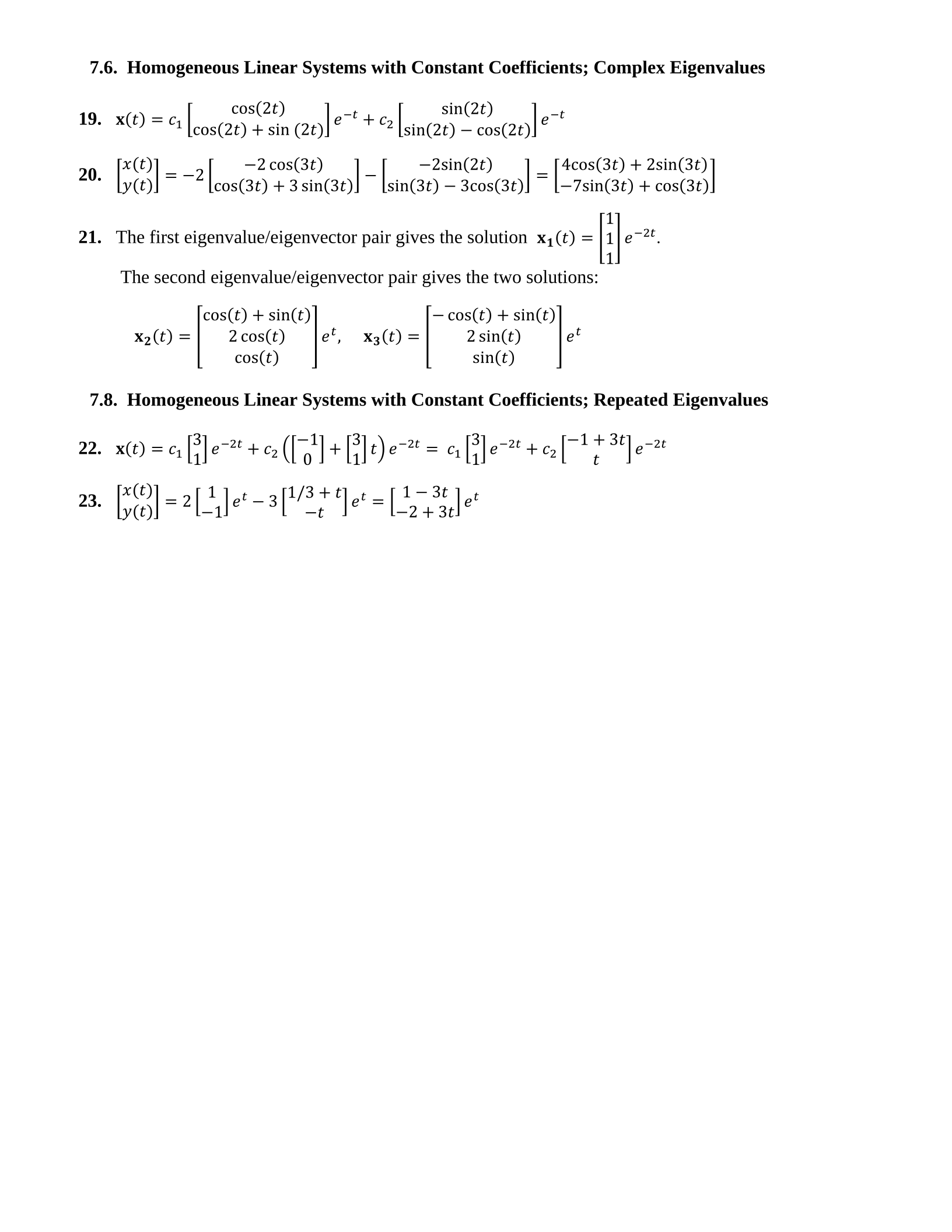
19. 𝐱(𝑡)=𝑐1[cos(2𝑡)
cos(2𝑡)+sin (2𝑡)]𝑒−𝑡+𝑐2[sin(2𝑡)
sin(2𝑡)−cos(2𝑡)]𝑒−𝑡
20. [𝑥(𝑡)
𝑦(𝑡)]=−2[−2cos(3𝑡)
cos(3𝑡)+3sin(3𝑡)]−[−2sin(2𝑡)
sin(3𝑡)−3cos(3𝑡)]=[4cos(3𝑡)+2sin(3𝑡)
−7sin(3𝑡)+cos(3𝑡)]
21. The first eigenvalue/eigenvector pair gives the solution 𝐱𝟏(𝑡)=[1
1
1]𝑒−2𝑡.
The second eigenvalue/eigenvector pair gives the two solutions:
𝐱𝟐(𝑡)=[cos(𝑡)+sin(𝑡)
2cos(𝑡)
cos(𝑡)]𝑒𝑡, 𝐱𝟑(𝑡)=[−cos(𝑡)+sin(𝑡)
2sin(𝑡)
sin(𝑡)]𝑒𝑡
7.8. Homogeneous Linear Systems with Constant Coefficients; Repeated Eigenvalues
22. 𝐱(𝑡)=𝑐1[3
1]𝑒−2𝑡+𝑐2([−1
0]+[3
1]𝑡)𝑒−2𝑡 = 𝑐1[3
1]𝑒−2𝑡+𝑐2[−1+3𝑡
𝑡]𝑒−2𝑡
23. [𝑥(𝑡)
𝑦(𝑡)]=2[1
−1]𝑒𝑡−3[1/3+𝑡
−𝑡 ]𝑒𝑡=[1−3𝑡
−2+3𝑡]𝑒𝑡
Powered by TCPDF (www.tcpdf.org)

