



MAT 275 - MATLAB #5
%% Lab 5 – Jose Cabrera - MAT 275 Lab
% Solution 1
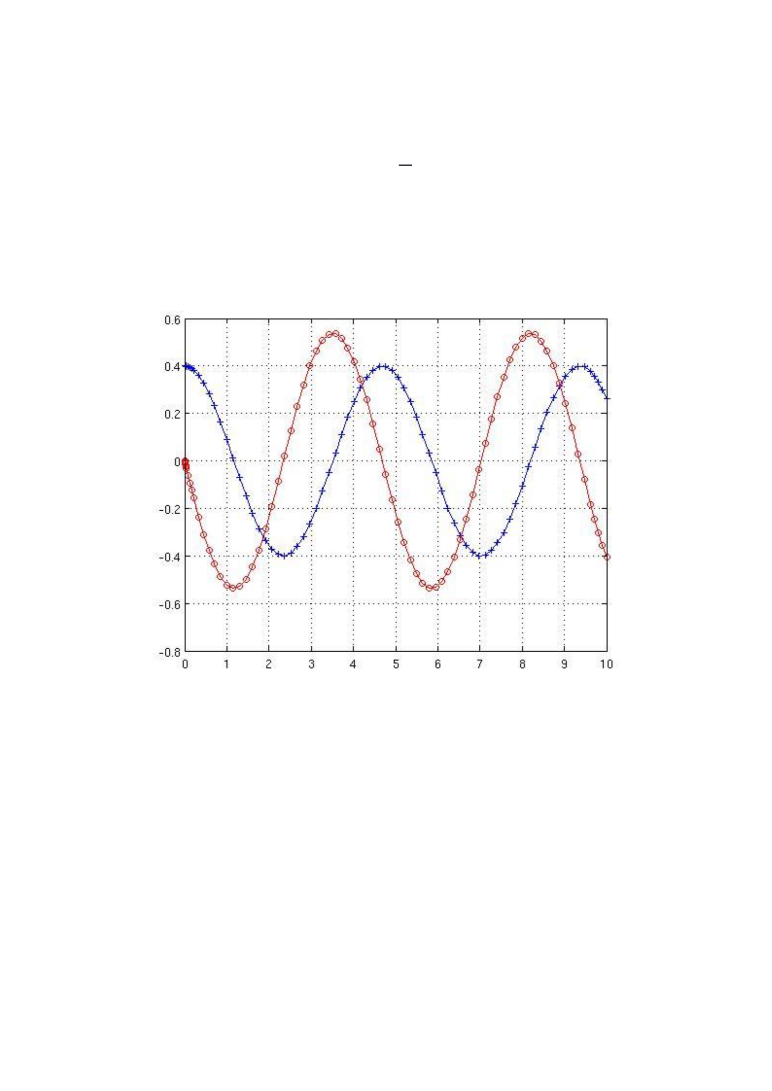
The curve in “blue” represents the equation y = y(t). Since according to the initial conditions in
LAB05ex1 the mass in the spring-mass system is displaced from its zero position. Clearly, the
curve in blue starts from at point 0.4 when t = 0. This signifies that the mass has some initial
displacement. The curve in red is at origin in the beginning which suggests that the velocity of the
mass is zero at t = 0.
% (B)
The curve y = y(t) is very similar to a sinusoidal curve. Thereby, inspecting the curve we can easily
calculate the time period.
By visual inspection the time period of the curve is approximately around 2.1s.
Analytically, we can use the equation relating the time period T and angular frequency ω
𝑇 = 2 ∗ 𝑝𝑖
𝜔
Here,
ω is equal to 3 rad/s
Hence, the time period T is equal to approx. 2.1s
% (C)
In the given system it is assumed that the damping forces are neglected. Due to this the mass will
continue to oscillate forever. Such a system is known as an ideal system as no damping forces (for
example air friction) are considered. As a result there is no force opposing the motion hence the
mass would continue to oscillate.
% (D)
From the graph it is evident that the curve in Blue is oscillating between the value +0.4 to -0.4. The
maximum displacement of the mass would be 0.4 cm.
% (E)
From the graph, the curve in Red is sinusoidal in nature and oscillates between the values +1.2 to -
1.2. Hence, the maximum velocity of the mass is also 1.2 cm/s.
All the time instants where the maximum velocity is attained by the mass -
Time (s)
0.540
1.55
2.644
3.677
4.74
5.736
6.786
7.835
8.883
9.948
% (E)
The following equation gives the relationship between spring constant (k), angular velocity and
mass(m) -
𝜔2=𝑘
𝑚
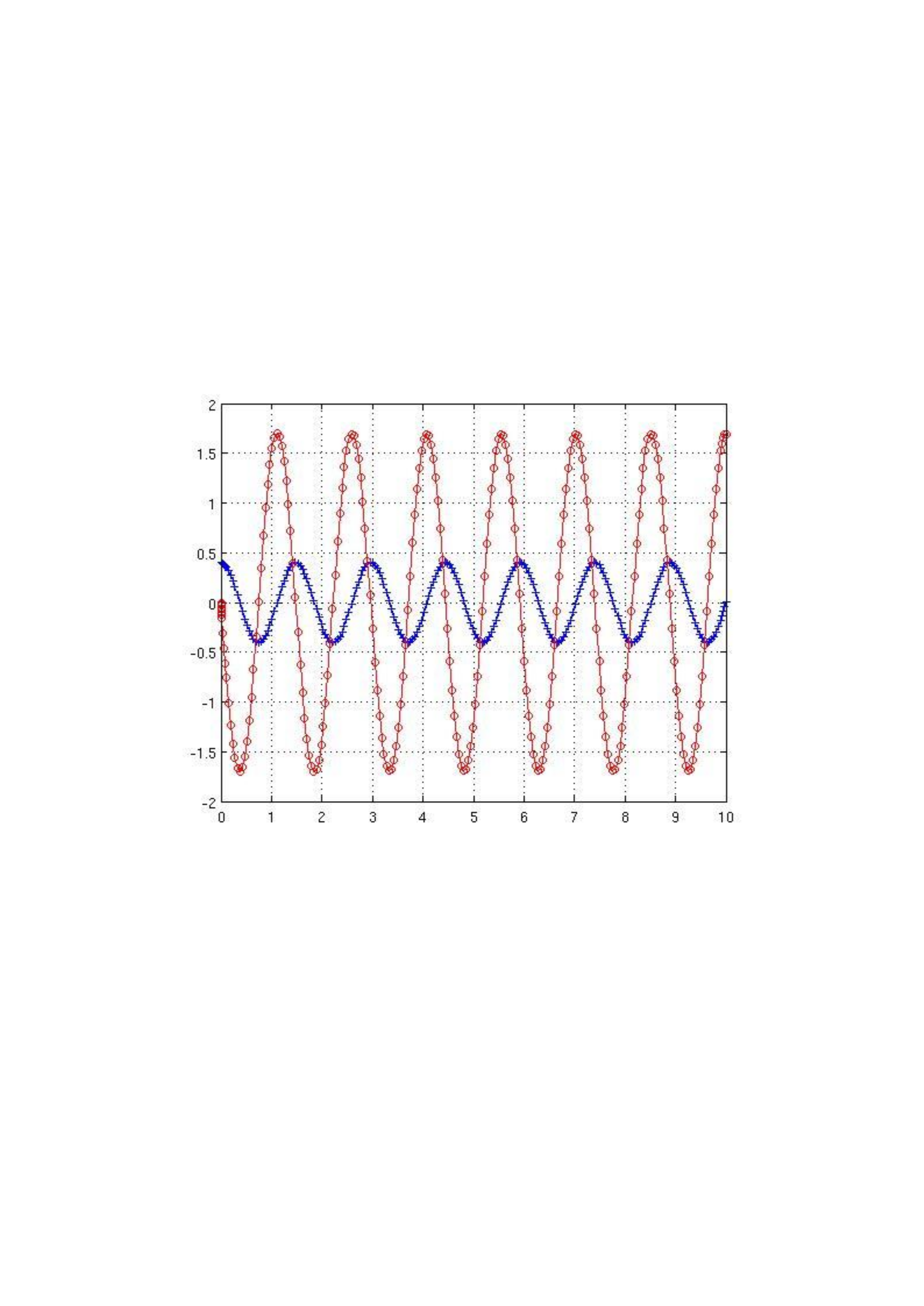
From part (B) we know that the time period is inversely proportional to the angular velocity.
Therefore we can conclude that the time period also depends on the spring constant and the mass.
Using the above equation as the mass “m” is increased it is expected that the time period should
also
increa
se.
The
follo
wing
graph
depict
s the
situati
on
when
m = 5
and k
= 9 -
Fig – m increased
Again when k increases it is expected that the time period should decrease.
The figure below is when m = 1 and k = 18:
Fig – k increased
% Solution 2
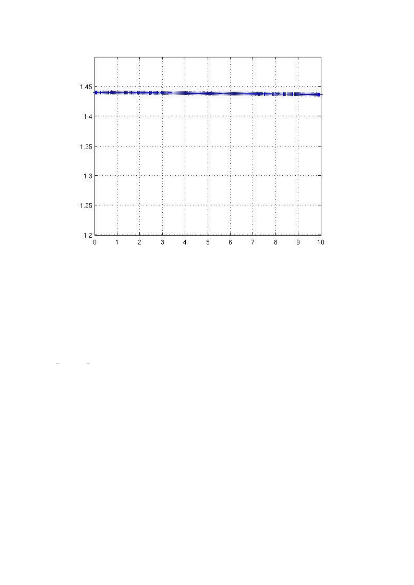
The graph of Energy against time is seen to represent a straight line (parallel to x-axis with y value
being constant at ~1.44).
This is true as in case when there are no damping forces present in the system, there is no energy
loss. The following plot confirms the same -
% (B)
Analytically, we can prove that the energy is constant and doesn't change with time by calculating
the derivative of E (which should come out to be 0).
Energy E:
𝐸 = 1
2𝑚𝑣2+1
2𝑘𝑦2
Differentiating with respect to time -
𝐸′ = 𝑚(𝑣 ∗ 𝑣′)+ 𝑘(𝑣 ∗ 𝑦′)
We know that :
v' = g
y' = v
𝐸′ = 𝑚(𝑣 ∗ 𝑔)+ 𝑘(𝑣 ∗ 𝑣)
𝐸′ = (𝑚𝑔 +𝑘𝑣)∗ 𝑣
From Equation L5.2
𝑚𝑔 = −𝑘𝑣
𝐸′ = 0as mg+kv=0
% (C)
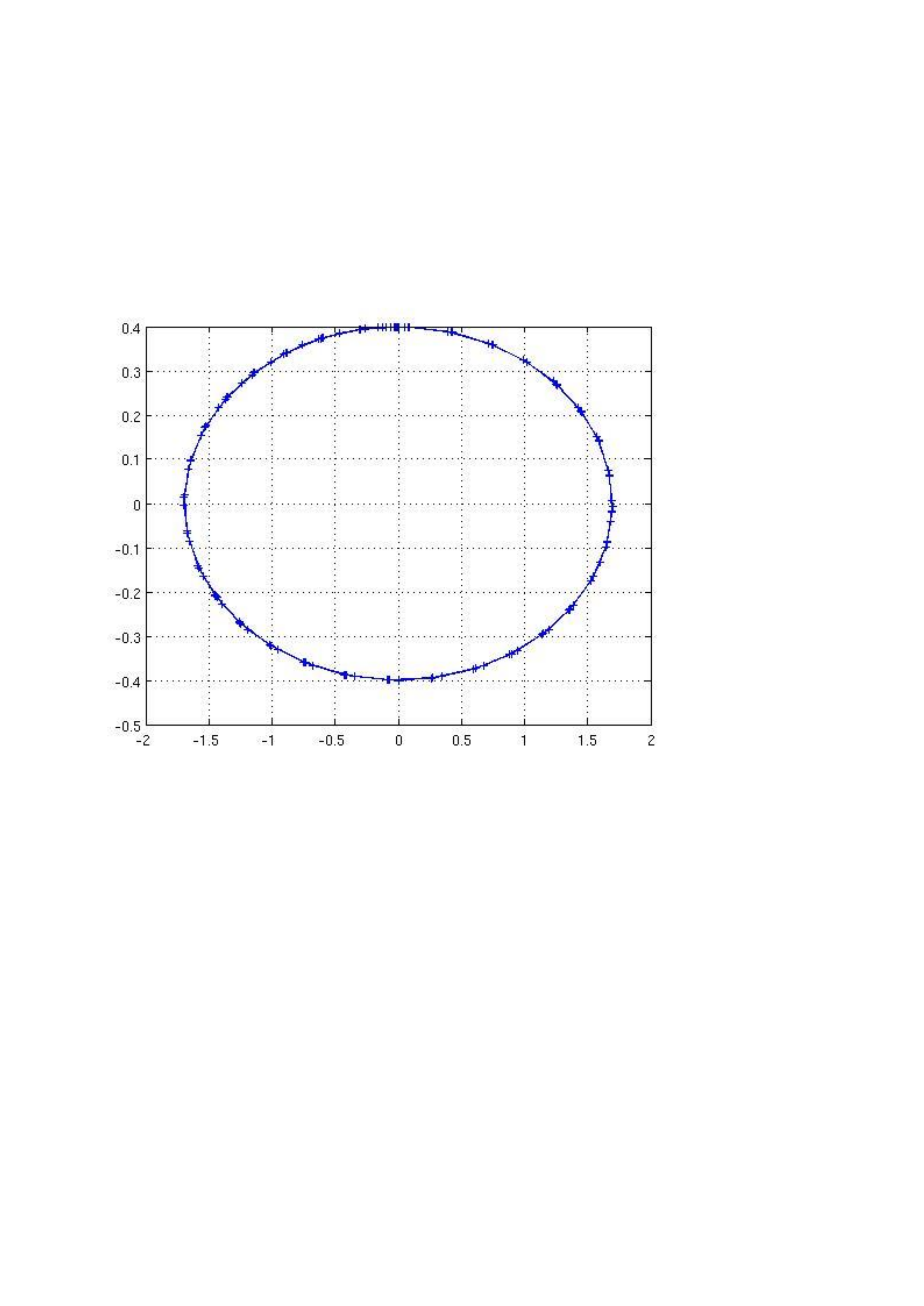
The phase plot should be circular in nature and thus it should never get closer to the origin. This is
expected since in case of ideal case there is a complete conversion from one form of energy to
other. The entire kinetic energy gets converted to spring energy and vice-versa. Therefore when the
displacement is zero, velocity of the mass is maximum and when the mass is at maximum
displacement its kinetic energy is zero at that moment.
% Solution 3
Matlab gives the output as shown below:
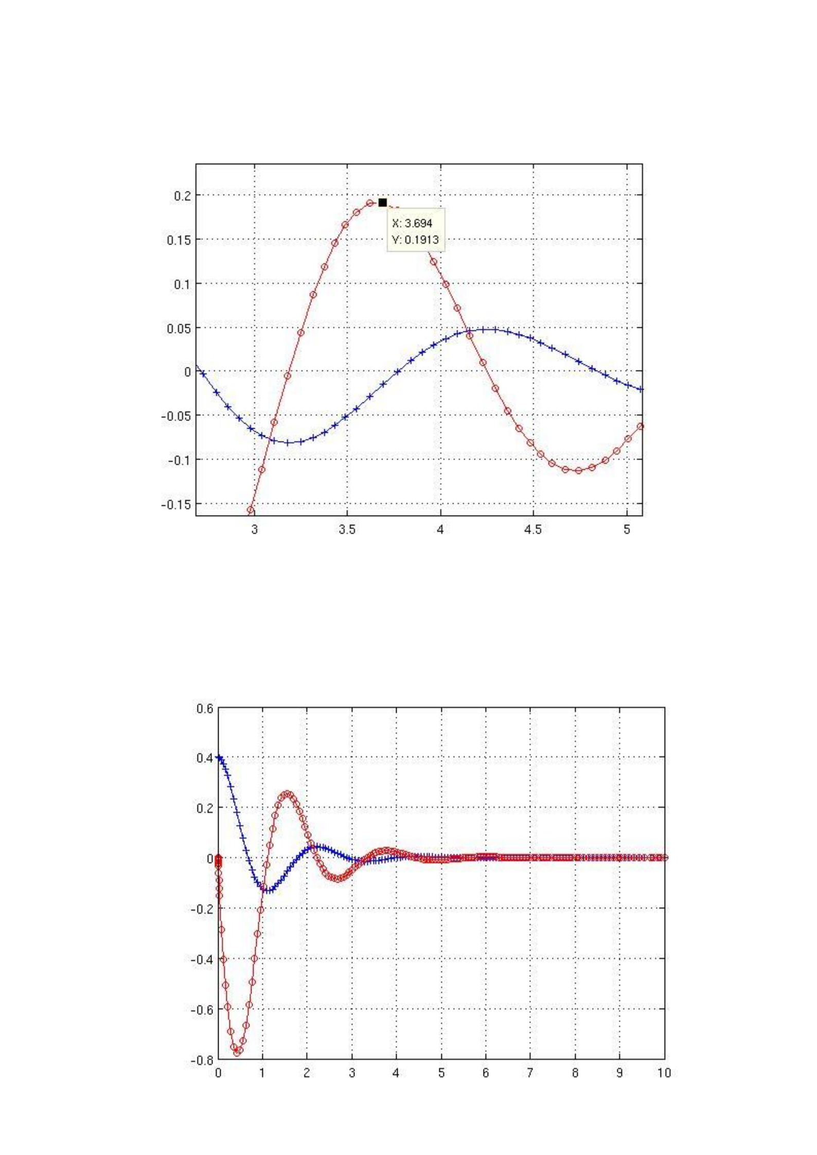
|y|<0.02 for t>t1 with 5.581<t1<5.6406
Here is the code for the same:
for iter=1:length(y)
% Get the max displacement every instant and store it in “k”
k(iter)=max(abs(y(iter:end)));
end
% Get the values of k < 0.01 using “find” function
k_min = find(k<0.02);
% Now minimum t is given by the first occurrence
k_min = k_min(1);
% “disp” to show output on screen
disp(['|y|<0.02 for t>t1 with ' num2str(t(k_min-1)) '<t1<'
num2str(t(k_min))]);
%
(B)
From the graph velocity comes out to be 0.191 cm/s (around t = 3.694 s)
% (C)
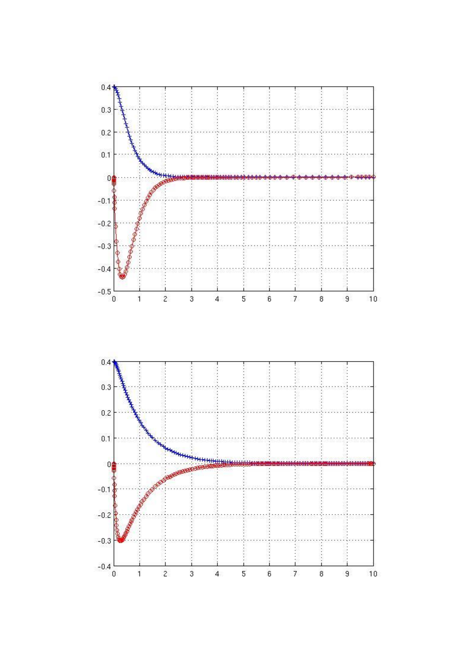
The following figures are obtained on varying c as 2, 4, 6 & 8
Fig c = 2
Fig
c= 6

Fig c= 10
From the graphs it is evident that as “c” increases the effect of damping forces increases.
Since damping forces are increasing the maximum displacement attained by the mass reduces. Also
the masss comes to rest after oscillating for some time.
% (D)
For a second order differential equation, in the case of “Critical Damping” there are no
oscillations. At critical damping we have two equal real roots of the characteristic equation.
The value of “c” is calculated mathematically below:
The concerned ODE is - ((all the terms have their usual meaning))
𝑚𝑦′′ + 𝑐𝑦′ + 𝑘𝑦 = 0
Initial conditions:
y(0) = yo, y’(0) = vo
The characteristic equation is-
λ2 + 2ᶓωλ + ω2 = 0
The roots of the characteristic equation:
λ = - ᶓω ± ω (ᶓ2 – 1) ½
In case of critical damping ᶓ is equal to 1 (required for two equal real roots).
Now,
ᶓ = 1 & ω = 3
c = 2ᶓω => c = 6
Same value of c can be found by inspecting the graphs.
% Solution 4
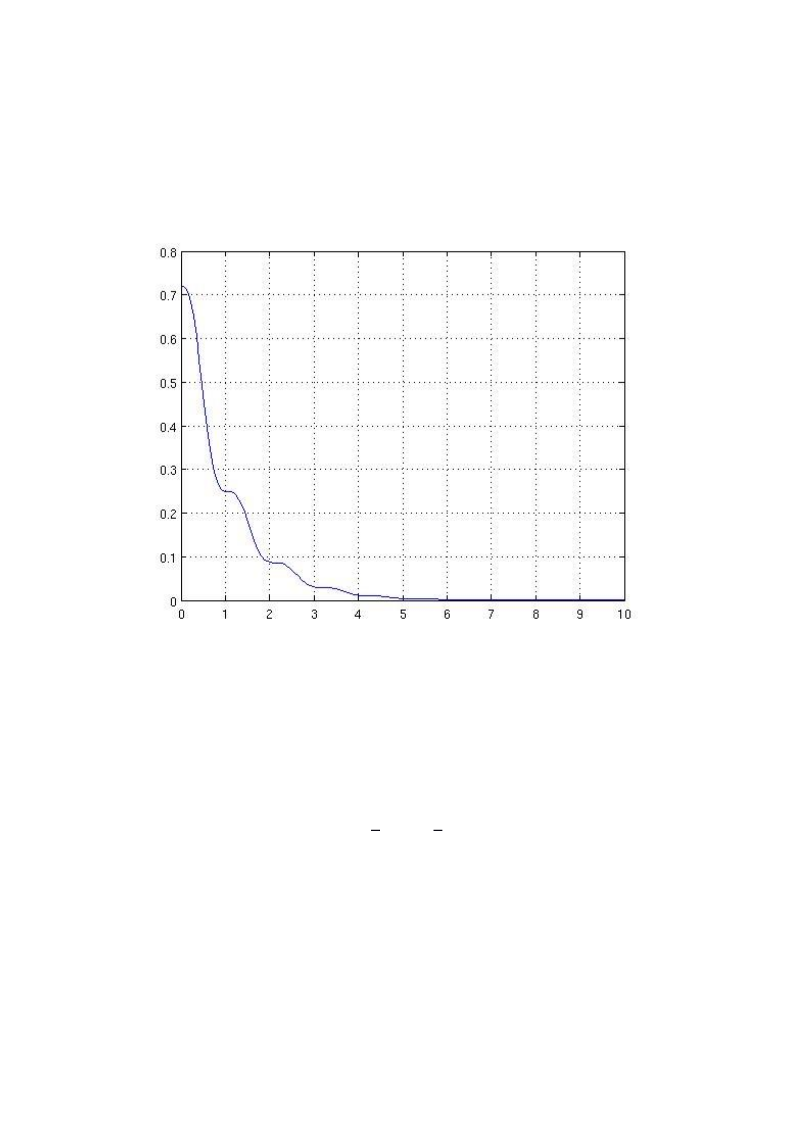
The graph between energy and time with the effect of damping forces is shown below:
As it can be seen that the Energy is not constant. As a result the energy is not conserved.
Since the energy goes to zero after certain period hence the spring-mass system doesn't retain all it's
energy but slowly looses it.
% (B)
The energy E of the spring-mass system is define as:
𝐸 = 1
2𝑚𝑣2+1
2𝑘𝑦2
The derivative with respect to time:
𝐸′ = 𝑚(𝑣 ∗ 𝑣′)+ 𝑘(𝑣 ∗ 𝑦′)
Also,
v' = g
y' = v
Using the above -
𝐸′ = 𝑚(𝑣 ∗ 𝑔)+ 𝑘(𝑣 ∗ 𝑣)
From Equation L5.4
𝑚𝑔 = −𝑘𝑣 − 𝑐𝑣
𝐸′ = −𝑐𝑣[Using L5.4]
Since E' and c have different signs as a result when c < 0 we have E' < 0 and vice-versa.
% (C)
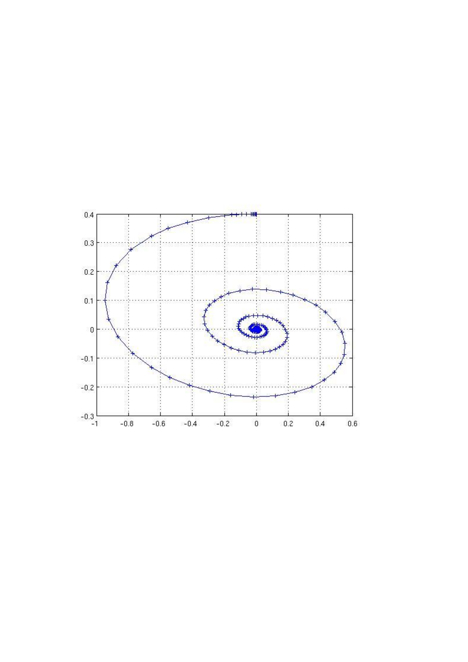
The phase plot between v and y with the effect of damping is shown below:
Fig – Phase Plot
The plot gets closer to the origin. This suggests that due to the effect of damping forces the Energy
is not conserved.
When the plot is at the origin the spring-mass system has lost all its energy. At this instant
displacement is zero as well as the velocity is zero. The spring mass system doesn't have either
kinetic or spring energy. Not all the kinetic/spring energy is converted into spring/kinetic energy.

