


MAT 275 MATLAB Assignment #4 NAME:____Allison Liaiga ______
LAB DAY and TIME:_ F @ 8:25_
Instructor: ______ England _____
Exercise 1a
type('LAB04ex1.m')
function LAB04ex1
t0=0; tf=50; y0=[-0.5,0.5];
[t,Y]=ode45(@f,[t0,tf],y0,[]);
y=Y(:,1);
v=Y(:,2);
figure(1);
plot(t,y,'b'); ylabel('y');
hold on
plot(t,v,'r'); ylabel('v');
ylim([-1.2,1.2]);
grid on
legend('y(t)','v(t)=y"(t)');
figure(2);
plot(y,v,'k');xlabel('y');ylabel('v=y"');
grid on
ylim([-1.5,1.5]);
xlim([-0.5,1]);
end
function [ dYdt ] = f( t,Y )
y=Y(1); v=Y(2);
dYdt=[v;sin(t)-7*v-5*y];
end
Exercise 1c
%As y goes to infinity it will keep oscillating as there seems to be no
%evidence of dampening. The amplitude and frequency seem to remain
%relatively consistent.
Exercise 1d
type('LAB04ex1d.m')
LAB04ex1d
%The long term behavior of the solution stays the same. The first plot
%still oscillates to infinity with the same values and consistency. The
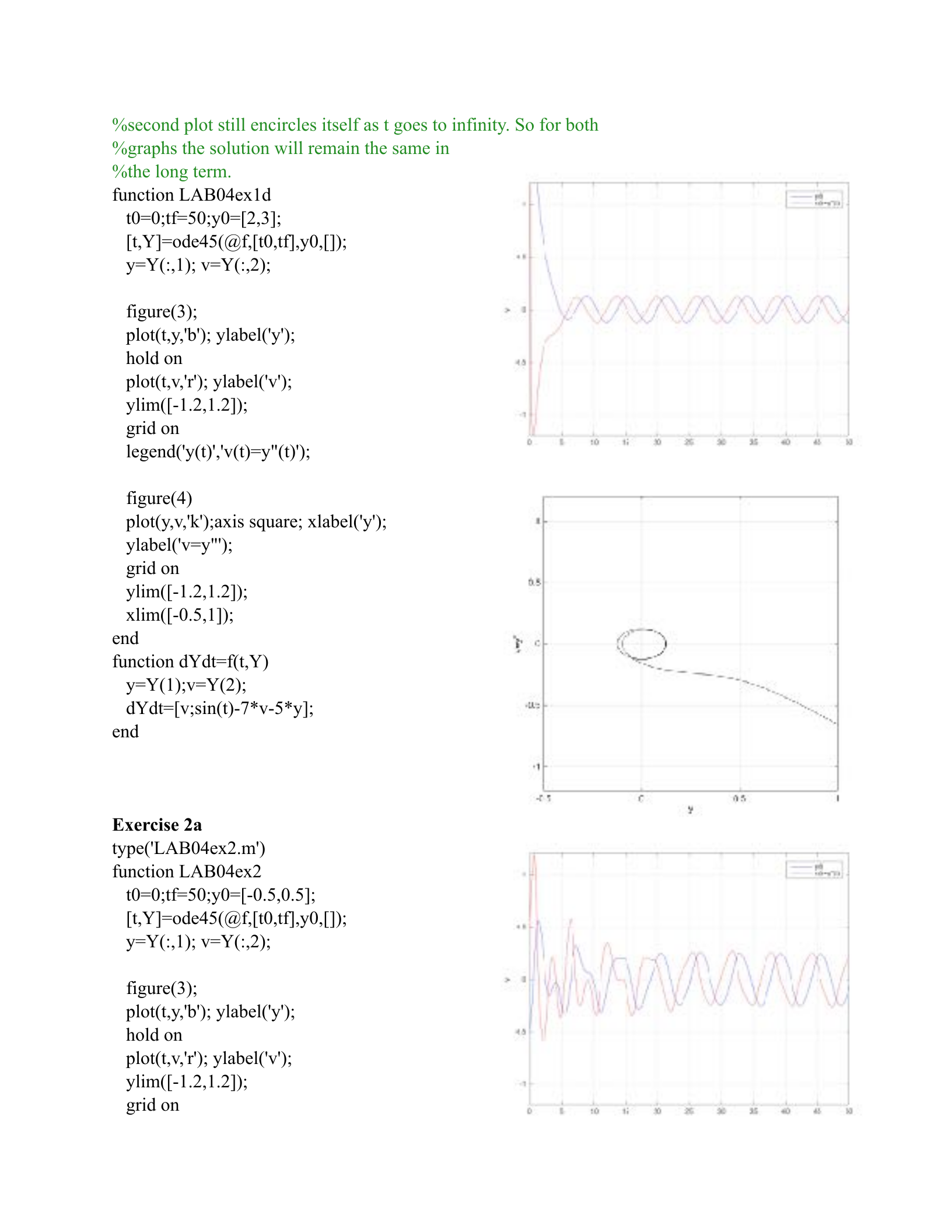
%second plot still encircles itself as t goes to infinity. So for both
%graphs the solution will remain the same in
%the long term.
function LAB04ex1d
t0=0;tf=50;y0=[2,3];
[t,Y]=ode45(@f,[t0,tf],y0,[]);
y=Y(:,1); v=Y(:,2);
figure(3);
plot(t,y,'b'); ylabel('y');
hold on
plot(t,v,'r'); ylabel('v');
ylim([-1.2,1.2]);
grid on
legend('y(t)','v(t)=y"(t)');
figure(4)
plot(y,v,'k');axis square; xlabel('y');
ylabel('v=y"');
grid on
ylim([-1.2,1.2]);
xlim([-0.5,1]);
end
function dYdt=f(t,Y)
y=Y(1);v=Y(2);
dYdt=[v;sin(t)-7*v-5*y];
end
Exercise 2a
type('LAB04ex2.m')
function LAB04ex2
t0=0;tf=50;y0=[-0.5,0.5];
[t,Y]=ode45(@f,[t0,tf],y0,[]);
y=Y(:,1); v=Y(:,2);
figure(3);
plot(t,y,'b'); ylabel('y');
hold on
plot(t,v,'r'); ylabel('v');
ylim([-1.2,1.2]);
grid on
legend('y(t)','v(t)=y"(t)');
figure(4)
plot(y,v,'k');axis square; xlabel('y');
ylabel('v=y"');
grid on
ylim([-1.2,1.2]);
xlim([-0.5,1]);
end
function dYdt=f(t,Y)
y=Y(1);v=Y(2);
dYdt=[v;sin(t)-7*v*y^2-5*y];
%change -7v to -7vy^2
end
Exercise 2b
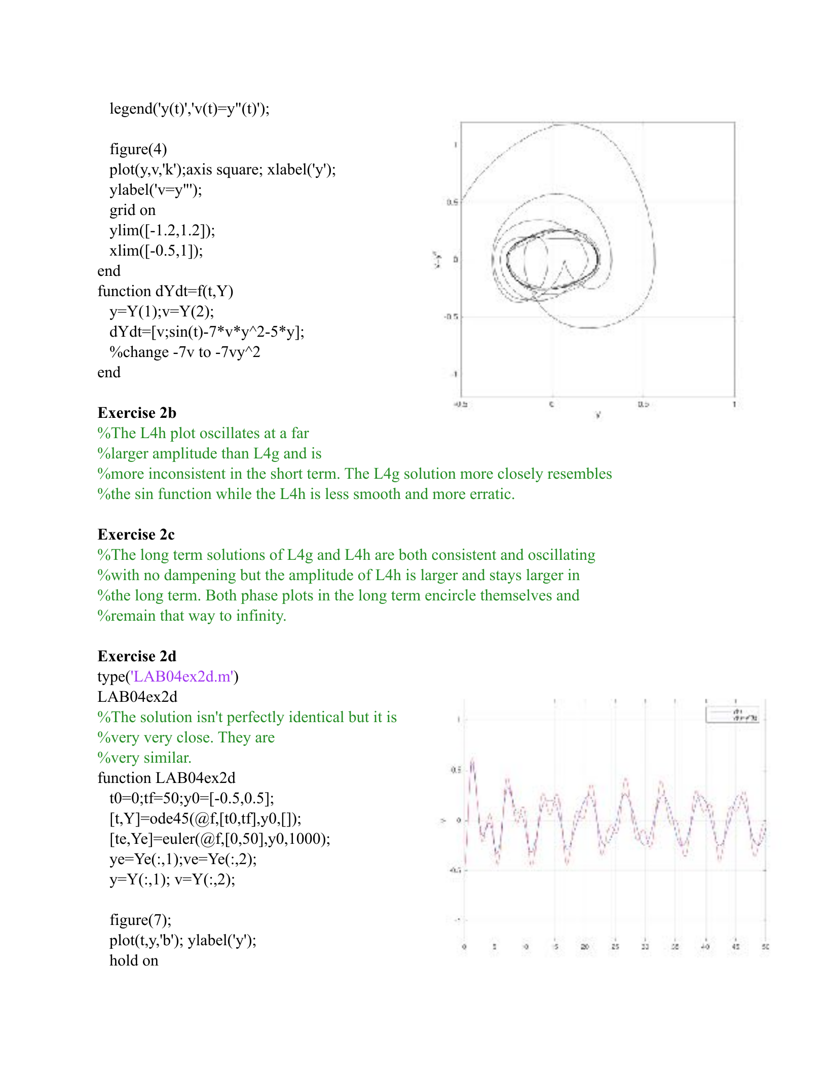
%The L4h plot oscillates at a far
%larger amplitude than L4g and is
%more inconsistent in the short term. The L4g solution more closely resembles
%the sin function while the L4h is less smooth and more erratic.
Exercise 2c
%The long term solutions of L4g and L4h are both consistent and oscillating
%with no dampening but the amplitude of L4h is larger and stays larger in
%the long term. Both phase plots in the long term encircle themselves and
%remain that way to infinity.
Exercise 2d
type('LAB04ex2d.m')
LAB04ex2d
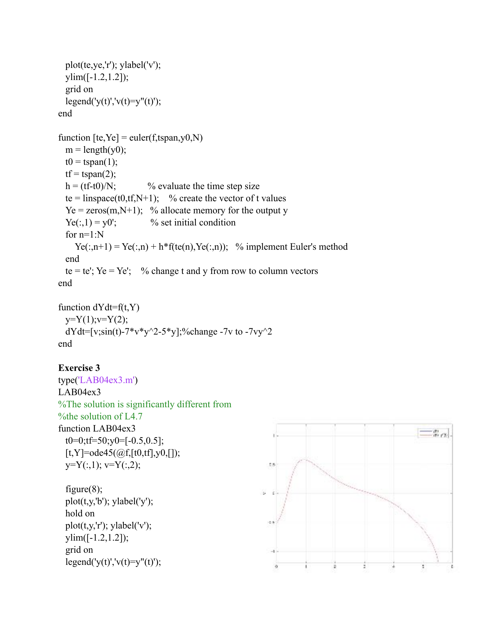
%The solution isn't perfectly identical but it is
%very very close. They are
%very similar.
function LAB04ex2d
t0=0;tf=50;y0=[-0.5,0.5];
[t,Y]=ode45(@f,[t0,tf],y0,[]);
[te,Ye]=euler(@f,[0,50],y0,1000);
ye=Ye(:,1);ve=Ye(:,2);
y=Y(:,1); v=Y(:,2);
figure(7);
plot(t,y,'b'); ylabel('y');
hold on
plot(te,ye,'r'); ylabel('v');
ylim([-1.2,1.2]);
grid on
legend('y(t)','v(t)=y"(t)');
end
function [te,Ye] = euler(f,tspan,y0,N)
m = length(y0);
t0 = tspan(1);
tf = tspan(2);
h = (tf-t0)/N; % evaluate the time step size
te = linspace(t0,tf,N+1); % create the vector of t values
Ye = zeros(m,N+1); % allocate memory for the output y
Ye(:,1) = y0'; % set initial condition
for n=1:N
Ye(:,n+1) = Ye(:,n) + h*f(te(n),Ye(:,n)); % implement Euler's method
end
te = te'; Ye = Ye'; % change t and y from row to column vectors
end
function dYdt=f(t,Y)
y=Y(1);v=Y(2);
dYdt=[v;sin(t)-7*v*y^2-5*y];%change -7v to -7vy^2
end
Exercise 3
type('LAB04ex3.m')
LAB04ex3
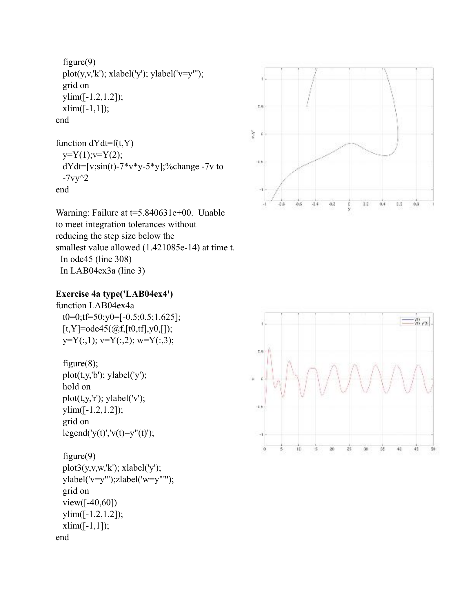
%The solution is significantly different from
%the solution of L4.7
function LAB04ex3
t0=0;tf=50;y0=[-0.5,0.5];
[t,Y]=ode45(@f,[t0,tf],y0,[]);
y=Y(:,1); v=Y(:,2);
figure(8);
plot(t,y,'b'); ylabel('y');
hold on
plot(t,y,'r'); ylabel('v');
ylim([-1.2,1.2]);
grid on
legend('y(t)','v(t)=y"(t)');
figure(9)
plot(y,v,'k'); xlabel('y'); ylabel('v=y"');
grid on
ylim([-1.2,1.2]);
xlim([-1,1]);
end
function dYdt=f(t,Y)
y=Y(1);v=Y(2);
dYdt=[v;sin(t)-7*v*y-5*y];%change -7v to
-7vy^2
end
Warning: Failure at t=5.840631e+00. Unable
to meet integration tolerances without
reducing the step size below the
smallest value allowed (1.421085e-14) at time t.
In ode45 (line 308)
In LAB04ex3a (line 3)
Exercise 4a type('LAB04ex4')
function LAB04ex4a
t0=0;tf=50;y0=[-0.5;0.5;1.625];
[t,Y]=ode45(@f,[t0,tf],y0,[]);
y=Y(:,1); v=Y(:,2); w=Y(:,3);
figure(8);
plot(t,y,'b'); ylabel('y');
hold on
plot(t,y,'r'); ylabel('v');
ylim([-1.2,1.2]);
grid on
legend('y(t)','v(t)=y"(t)');
figure(9)
plot3(y,v,w,'k'); xlabel('y');
ylabel('v=y"');zlabel('w=y""');
grid on
view([-40,60])
ylim([-1.2,1.2]);
xlim([-1,1]);
end
function dYdt=f(t,Y)
y=Y(1);v=Y(2);w=Y(3);
dYdt=[v;w;cos(t)-7*w*y^2-14*y*v^2-5*v];
end
Exercise 4b
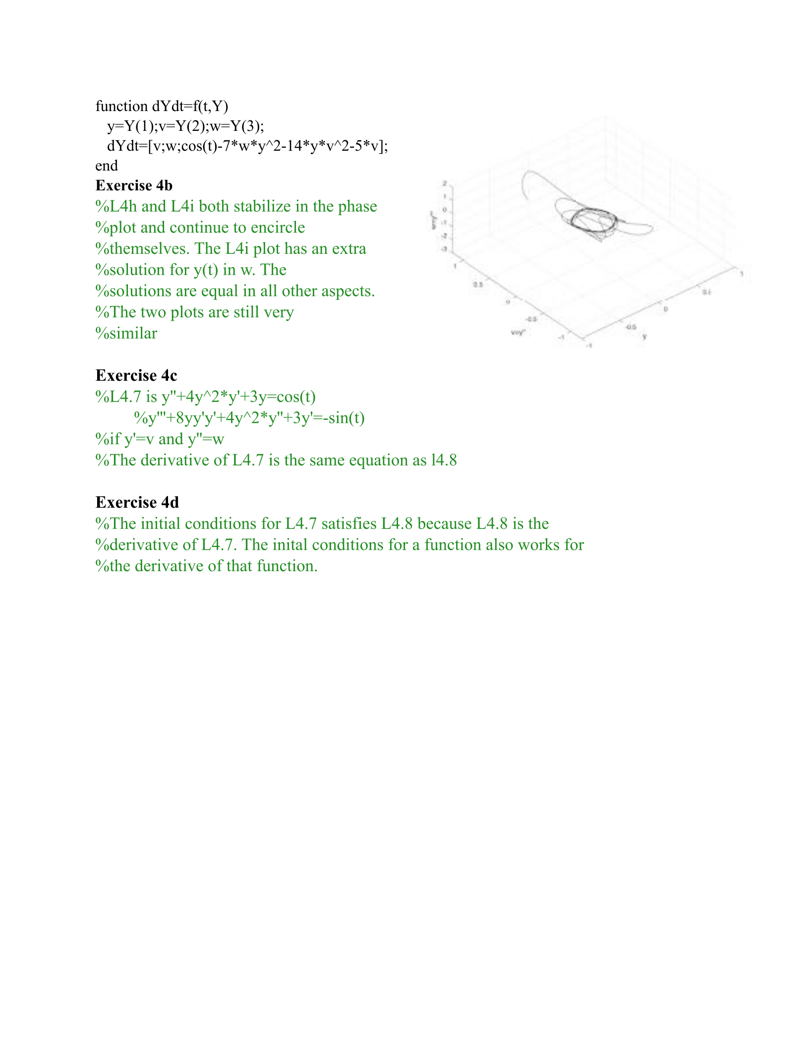
%L4h and L4i both stabilize in the phase
%plot and continue to encircle
%themselves. The L4i plot has an extra
%solution for y(t) in w. The
%solutions are equal in all other aspects.
%The two plots are still very
%similar
Exercise 4c
%L4.7 is y''+4y^2*y'+3y=cos(t)
%y'''+8yy'y'+4y^2*y''+3y'=-sin(t)
%if y'=v and y''=w
%The derivative of L4.7 is the same equation as l4.8
Exercise 4d
%The initial conditions for L4.7 satisfies L4.8 because L4.8 is the
%derivative of L4.7. The inital conditions for a function also works for
%the derivative of that function.
Powered by TCPDF (www.tcpdf.org)

